Submicrosecond timing on ESP32 with passive BLE
Capturing the right event, tracking clock drift and checking predictions brought passive BLE timing into the tens of nanoseconds on a measured ESP32-S3 path.
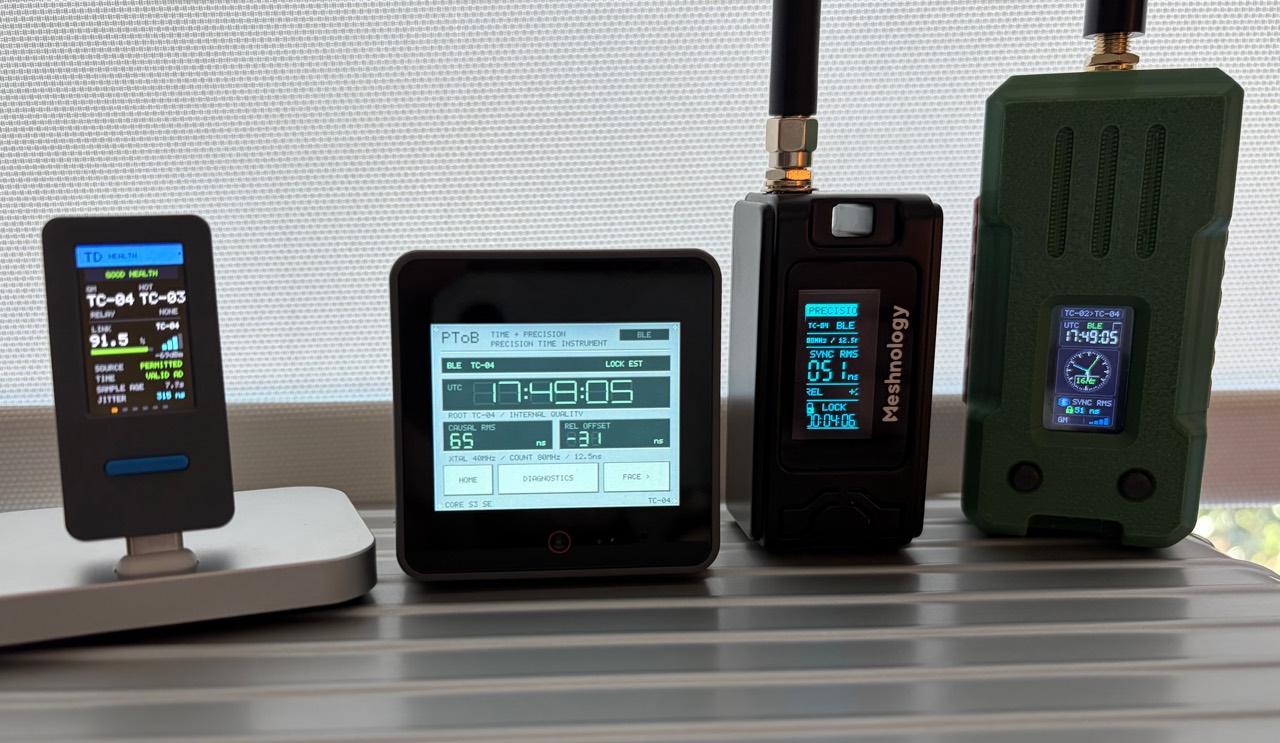
An inexpensive ESP32 board can keep surprisingly close time with a radio source simply by listening. Our latest PToB measurements on the ESP32-S3 W12 recorded 60.3 ns RMS relative timing error across 522 usable observations out of 600 logged. The largest usable error was 180 ns, well below one microsecond, or 1,000 ns. The other 78 observations were unavailable during a source transition and remain part of the result.
The timing arrives over passive BLE reception. The receiver listens to broadcast timing packets and their follow-up corrections, then maintains its own clock between updates. It does not need a request-and-response exchange for each timing measurement.
Getting there meant working around an architecture built to deliver packets conveniently to applications. Precision timing asks a more demanding question: exactly when did the relevant event happen?
Why passive reception matters
A broadcast can serve many listeners. Adding another receiver does not require another individual timing exchange with the source. That is an appealing foundation for sensors and instruments that need a shared sense of time across a room or a local mesh.
Here, “passive” describes how the receiver obtains its timing observations. PToB also has authenticated admission and renewal traffic, and a relay transmits its own timing stream. The claim is about the broadcast timing path, rather than a promise that every device stays radio silent throughout its lifetime.
This architecture avoids per-listener timing replies. Its eventual capacity and energy use still need measurement; a continuously listening radio has a cost of its own.
The callback arrives after the event
The obvious implementation is to read the local clock when the Bluetooth stack reports a packet. That records when software handled the message. Radio processing, interrupts, queues and other work can all sit between reception and that callback. Their delays vary.
There is also more than one clock inside the chip. The Bluetooth controller schedules radio activity in one coordinate system, while local peripherals count in another. Two readings can both be precise and still describe different moments. Meanwhile, the receiver’s oscillator runs a little faster or slower than the source, so a one-time correction soon becomes stale.
These effects become substantial when the entire error budget is a fraction of a microsecond. Printing more decimal places cannot recover timing information lost along the way.
Capture the event and match the packet
Our fine receive path uses a hardware capture peripheral to latch a radio receive-active transition against a continuously running 80 MHz counter. Software can collect that saved count later. The counter’s 12.5 ns ticks give us a fine measuring grid; they do not guarantee 12.5 ns accuracy.
The next challenge is attaching that transition to the correct packet. BLE traffic can include repeated copies, different channels and unrelated activity. We retain the packet information and require an unambiguous match. A missing or ambiguous match produces an unavailable observation instead of a plausible-looking timestamp.
The captured marker also needs a consistent relationship to the packet’s timing convention. We use a packet-specific empirical adjustment. The precise RF endpoint and its physical delay remain unqualified, which matters when transferring the technique to another board or packet format.
Keep the clocks connected
The receiver builds a model of how its counter relates to the source clock: how far ahead or behind it is, and how quickly that difference changes. This is the job of the software phase-locked loop, or Software PLL. Repeated observations keep that relationship current, while controlled adjustments steer the delivered clock.
Channel differences need care too. If one BLE channel has a slightly different timing offset, a changing mix of channels should not look like an oscillator suddenly speeding up. The estimator accounts for that distinction when learning the clock’s rate.
Crossing between internal clocks needs equally careful handling. We bracket a clock read with two local counter captures, keeping the interval short and recording its width. The critical instructions run from internal RAM to reduce variation from flash access. That gives us a measured clock bridge rather than an assumption that two software reads were simultaneous.
The implementation paper covers the counter rollover rules, capture association, clock bridges and fitting equations. At the architectural level, the solution is straightforward: preserve the original event, translate between clocks carefully and keep tracking drift.
Check the clock that was actually available
A timing model can look excellent if it is allowed to learn from an observation before being scored against it. We preserve the prediction available at capture and score it before the later correction updates the model.
For the delivered-clock check, a physical GNSS pulse-per-second signal acts as a witness. At each captured pulse, we query the BLE clock that was already available. The witness does not train the BLE clock. This tests the receiver’s delivered relative time, beyond the estimator’s own internal fit score.
The current 24 October baseline contains two declared five-minute windows after a two-minute warmup. Its empirical adjustments were frozen beforehand, with no final-window refit or removal of large errors.
| Observation | Usable / logged | RMS | Max error |
|---|---|---|---|
| W12, both windows | 522 / 600 | 60.3 ns | 180 ns |
| W12, stable second window | 300 / 300 | 38.3 ns | 121 ns |
| Through the W12 relay | 451 / 600 | 61.9 ns | 211 ns |
RMS summarizes the errors across the usable observations, including any persistent offset. The maximum is the largest absolute error observed; neither predicts a guaranteed bound for the next run.
The first window changed sources and retained 78 unavailable W12 observations. The downstream measurement has its own 149 unscorable records. Submicrosecond precision when a valid clock is available and continuous availability are separate engineering goals.
These are relative-PPS measurements on the tested paths. Calibrated UTC accuracy, physical output-pin timing and transfer to other units remain open work. The implementation paper retains its earlier experiments; the later baseline above has its own public evidence and measurement rows.
How this compares with active Wi-Fi FTM
An impressive comparison is Alexandre Bezroutchko’s Fine Time Sync project. It uses Wi-Fi Fine Timing Measurement, or FTM, to relate ESP32 clocks and discipline hardware timers. The project reports output jitter below 100 ns, with 25 ns timer adjustment granularity.
That is a slightly tighter headline output figure than the 121 ns maximum relative error in our stable BLE receive window. The measurements describe different endpoints: FTS reports hardware pulse jitter, while our result measures a delivered clock against captured PPS. They establish a similar scale of timing performance, rather than a controlled ranking of clock accuracy.
The architectural difference is substantial. FTM exchanges frames in both directions and timestamps their departure and arrival in hardware. Its round-trip observations provide information about link delay; the FTS design uses them to build a clock relationship and align timer events.
Our BLE receiver obtains timing from the source’s broadcast stream. It has no equivalent per-observation round-trip measurement, so propagation and fixed radio delays remain part of the uncertainty and empirical path adjustment. In return, multiple receivers can consume the same stream without each negotiating a timing exchange.
Active FTM offers a strong route to synchronized hardware pulses. Passive BLE offers a different distribution architecture, with measured relative timing already in the same broad submicrosecond range. The interesting result is how much precision we can recover from listening carefully.
What comes next
The remaining work is to make that precision dependable across source changes, more boards and longer observations. Relay transmit time is still estimated from controller scheduling and clock maps; a verified physical transmit timestamp would give us a firmer foundation. Reference delays, temperature, load and calibration transfer also need their own measurements.
For now, an ESP32-S3 running our fine-capture firmware has demonstrated tens-of-nanoseconds RMS relative timing over a passive BLE receive path. The research paper explains the machinery, and the current results keep the errors and gaps visible alongside the headline numbers.