Building a basic ESP32 clock
Our first ESP32 firmware example shows how to turn ticks into time, correct a clock that runs fast and catch up without making its reading jump.
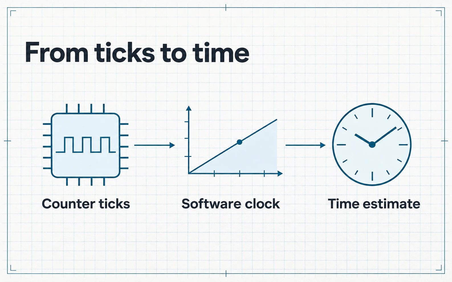
Set two clocks to the same time and come back later. If one has pulled ahead, setting it again will bring them together for a moment. To keep them together, you also have to change how fast that clock advances.
That is the idea behind clock discipline: use a reference to bring a clock’s reading and its pace into agreement. We start our ESP32 firmware series with Example 00: Clock fundamentals. It runs on your computer with simulated inputs, so you can see what each correction does before adding an ESP32 board, a radio or a UTC reference.
Turn counter ticks into time
A counter tells you how many ticks have passed. To turn that count into time, software needs a starting point where a particular tick has a known time, and a rate for converting later ticks into elapsed time. The example uses a simulated 80 MHz counter and starts from a relative time of zero.
The counter can wrap to zero while time keeps moving. The lesson follows a count across that boundary and keeps the ticks on a continuous timeline. It also shows why keeping raw ticks matters: at the nominal rate one tick is 12.5 nanoseconds, so rounding each tick separately loses information. A timestamp can be written in nanoseconds even when the clock’s accuracy is much coarser.
Correct the pace
In the lesson, the simulated counter runs 20 parts per million fast. That is 20 extra microseconds of clock error every second if software keeps using the nominal conversion. After ten seconds, the clock is 200 microseconds ahead.
The example supplies a known correction. Software assigns slightly less time to each tick, so the estimate advances at nearly the reference rate. The oscillator keeps running as before. A later lesson will estimate the correction from observations.
Catch up without a jump
Two clocks can run at the same pace and still disagree. The difference between their readings is called phase error. If the software clock is behind, it can advance a little faster until it catches up, then return to its usual pace. This gradual adjustment is called a slew. If the clock is ahead, it can slow down while still moving forward.
In the lesson, a clock starts two microseconds behind. It reads the same value just before and just after the update. Over the next two seconds it makes up the difference. That continuity matters when another part of your program uses the clock to order events or measure intervals.
Keep the reading you had at the time
Sometimes the reference time for an event arrives after the event itself. Save the clock’s prediction when the event happens. When the reference value arrives, compare it with that saved prediction before applying the correction. That tells you how well the clock was doing when your program needed it.
A clock also needs to say when it has no usable reading. In Example 00, a read at the deadline is refused, even if you recently adjusted the clock. A timing correction does not extend that deadline. A counter can also become unreliable if you wait so long between reads that you can no longer tell how far it advanced.
Take the same questions to the board
When you move from simulation to a board, open the ESP32-S3 timing schematic. It follows the W12 implementation from the local timebase and event capture through to the software clock. Select a block to see what to check there. If the error grows steadily, start with the raw tick intervals and their conversion rate. If timestamps vary when the system gets busy, check whether you recorded when the event happened or when software got around to handling it. If time disappears after a restart or a gap, check counter continuity and whether the clock still has a usable reference.
To get a feel for the difference between rate and phase, run Example 00 on your computer and reverse the sign of the rate correction. Predict which way the error will grow before you run it again. In Part 2, the clock learns the correction from Bluetooth observations. Sync ESP32 sensors over BLE